Equal Truck Loads in Vehicle Routing: A Measured Case Study

Would you send out a truck that is only 44% full?

Five trucks. 31 destinations. 410 crates of sparkling water to deliver.

The trucks leave with 98, 98, 44, 98 and 72 crates, despite each having room for 100. On a dispatch screen, one loading bar looks like a problem. The obvious reaction is tempting: “Move some deliveries. Balance the trucks.”

In Why a Less-Loaded Truck Can Make Sense, we explained why that reaction needs a whole-plan calculation. That follow-up to our CVRP worked example left a practical question open: what happens if equal departure loads become a requirement, rather than a preference?

This article tests it. We keep the published 784-unit plan as our baseline and require all five trucks to depart with 82 crates each. OptAlgo found a verified plan traveling 920 benchmark units, 136 units, or 17.35%, farther. Fleet-wide departure utilization? Still 82%.

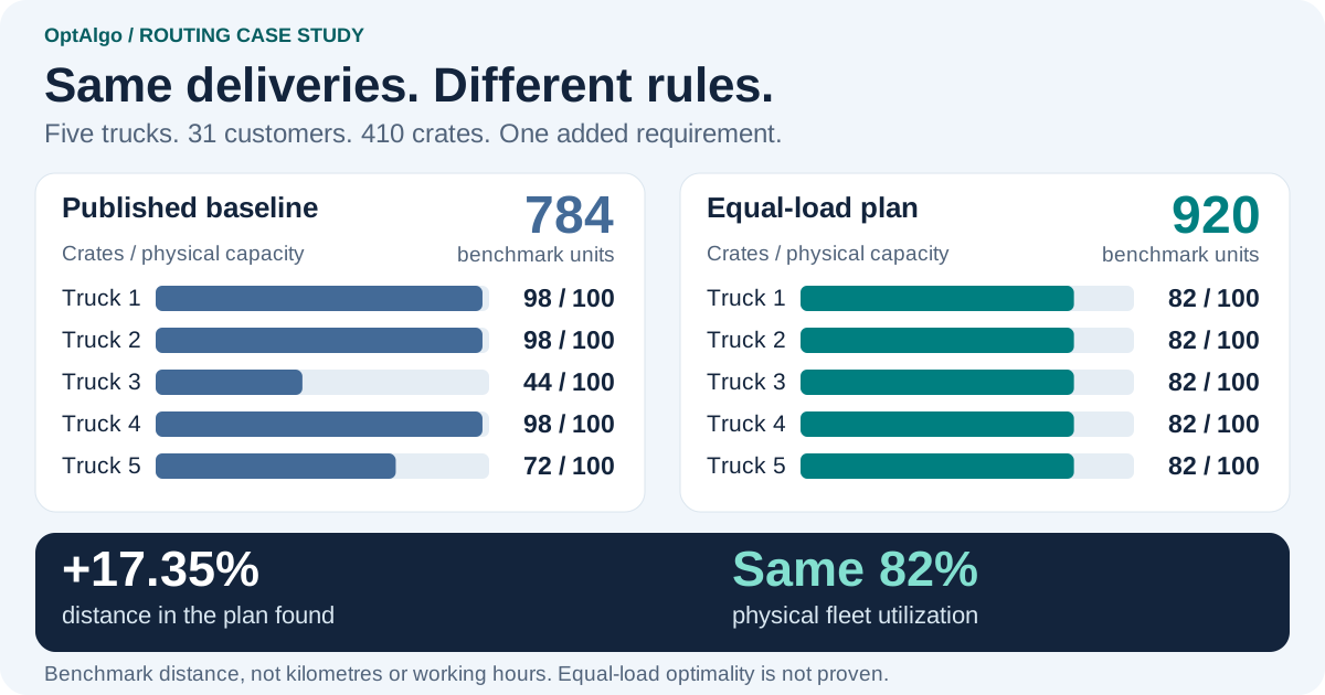
Figure 1. Same demand and physical fleet; a different dispatch rule. The 17.35% increase compares the two plans. The equal-load optimum is not yet proven.

The point is not that balanced loading is a bad policy. It is that a better-looking loading chart and a better routing plan are different things. Here is the model behind the comparison, and what the evidence lets us conclude.

As in the earlier articles, European city names provide the delivery story. All numerical distances are academic benchmark units, not road distances, kilometres or working hours.

From “balance the trucks” to a precise business rule

“Balanced” can mean equal quantities, similar stop counts, or comparable driver hours. Those are different requirements. For this experiment, we choose one: exactly the same quantity on every departure.

The earlier load-utilization follow-up showed five loads of 82 as a hypothetical arithmetic split. It did not claim that the indivisible customer orders could form those routes. This experiment adds that requirement to the optimization and checks an actual solution.

Modeling choice	Original problem	Equal-load problem
Objective	Minimize total route distance	Unchanged
Orders and customer service	410 crates; each of 31 customers served once, without splitting an order	Unchanged
Fleet and trips	At most five depot-to-depot routes; one trip per truck	Unchanged
Physical truck capacity	100 crates	Unchanged: 100 crates
Operational route-load limit	At most 100 crates	At most 82 crates, which forces exactly 82 here
Depot and travel costs	Original benchmark depot and distance matrix	Unchanged
Load-balancing objective	None	None: equal loading is a hard requirement

Four original trucks could carry only 400 crates, so serving all 410 requires five. The equal split is 410 ÷ 5 = 82. The trucks do not shrink: we impose an 82-crate dispatch cap on vehicles that still physically hold 100.

This is not a soft penalty that the optimizer may trade against distance, nor a general “minimum 82 crates” feature. It is an instance-specific way to impose exact equality. The algebra explains why.

The mathematical models: one objective, two feasible sets

We can express both problems by selecting complete routes. This is a mathematical description of the routing decisions, not a software configuration.

Let N be the customer set and qᵢ the positive order quantity for customer i. A candidate route r starts and ends at the depot and visits a nonempty set of customers without repetition. Its load is Lᵣ, and its distance cᵣ includes both depot legs. Define:

Here Q is the operational load cap. R(Q) includes all candidate routes meeting that cap. Let aᵢᵣ = 1 when route r visits customer i, and zero otherwise; yᵣ = 1 means we select that route.

Both problems use this route-selection model:

In plain language: choose routes with the smallest combined distance, cover every customer exactly once, and use no more than five trucks. Capacity is already enforced by which routes are allowed into R(Q).

Problem 1: minimize distance with a 100-crate capacity ceiling

Set Q = 100. A truck may leave with any load up to 100 if the complete plan serves all orders within the fleet limit. Uneven loads are allowed. The published 98, 98, 44, 98, 72 plan is one such solution.

Problem 2: minimize distance while requiring equal departure loads

Set Q = 82, keeping everything else unchanged. For any complete feasible plan, let m be its number of routes and Lₖ the load on route k. Then:

Both ends equal 410, so every inequality must be tight: m = 5, and L₁ = L₂ = L₃ = L₄ = L₅ = 82. A route below 82 would leave demand that the other four could not absorb without exceeding the cap.

This proves what every feasible solution must look like, not that a feasible partition of whole customer orders exists. The verified routes below establish that existence for this instance.

Let F₁₀₀ and F₈₂ denote the complete feasible plans under the two caps, and D*₁₀₀ and D*₈₂ their minimum total distances. When equal loading is feasible, the relationship is:

Every equal-load plan is allowed in the original problem; the reverse is not true. Restricting the choices cannot improve the minimum distance under the same objective. It can leave that distance unchanged, increase it, or make the problem infeasible. The model does not assume a distance penalty; the results must establish it.

The original five-route plan

We retain the route numbering, customer groups, loads and distances from the published guide. Every order is delivered in one visit, and every route begins and ends at the Paris depot.

Published route	Delivery stops	Load in crates	Distance in benchmark units
1	8	98	230
2	10	98	267
3	2	44	59
4	7	98	155
5	4	72	73
Total	31	410	784

The 44-crate truck serves Brussels and London, contributing just 59 units to the total. Moving an order onto it changes both its route and the route that gives up the order, the whole-plan effect examined in the previous follow-up. Spare capacity alone does not tell us whether the reassignment helps.

A verified plan with 82 crates on every truck

The equal-load solution serves all 31 customers exactly once. All five routes start and end at the depot and carry exactly 82 crates. The saved customer sequences, order quantities and distances were independently checked against the retained input.

Equal-load route	Delivery stops	Load in crates	Distance in benchmark units
1	8	82	214
2	8	82	257
3	6	82	155
4	5	82	192
5	4	82	102
Total	31	410	920

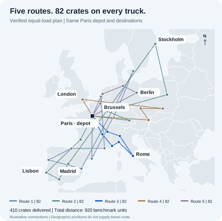
Figure 2. The equal-load requirement changes customer groupings and visit sequences. City positions match the original illustration. Travel costs come from the benchmark, not this map. Map data: Natural Earth.

Route numbers identify trips within each plan. Equal-load route 1 is not baseline route 1 with a different loading bar. Customers have moved between routes; the complete plan has changed.

More distance, but no increase in fleet utilization

Measure	Published baseline	Verified equal-load plan
Optimization budget	60 seconds	60 seconds
Trucks used / customers served	5 / 31	5 / 31
Physical capacity per truck	100 crates	100 crates
Departure loads	98, 98, 44, 98, 72	82, 82, 82, 82, 82
Fleet-wide departure utilization	82%	82%
Unused physical capacity	90 crates	90 crates
Total distance	784 benchmark units	920 benchmark units
Extra distance versus baseline	-	136 units / 17.35%

The calculations are deliberately separate:

Extra distance = 920 − 784 = 136 benchmark units
Percentage increase = 136 ÷ 784 × 100 ≈ 17.35%

Physical fleet utilization = 410 ÷ (5 × 100) × 100 = 82%
Unused physical capacity = 500 − 410 = 90 crates

Equal loading redistributes unused capacity; it does not eliminate it. The 82-crate dispatch cap must not replace the 100-crate physical capacity in the utilization denominator.

Both published runs had 60-second budgets, but they were separate runs. This is a comparison of verified plans, not a controlled solver-performance benchmark. Matching budgets alone do not establish identical execution conditions.

What the bound proves, and what remains open

The baseline matches the 784-unit known optimum of the original A-n32-k5 benchmark, as listed by CVRPLIB. That reference applies to the original model, not the equal-load variant.

The equal-load run reported a certified global lower bound of 902 and a verified plan at 920. It stopped at its 60-second search deadline without proving optimality. These two values bracket the equal-load optimum:

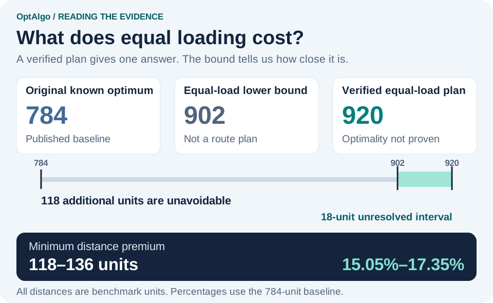
Figure 3. A lower bound is not a route plan. Together with a feasible plan, it limits what the best possible equal-load distance could be.

At least 118 extra units are unavoidable under this model. The 136-unit increase in the plan found is not all proven necessary. The minimum premium lies between approximately 15.05% and 17.35% of the baseline.

The remaining proof gap uses a different denominator:

Proof gap = (920 − 902) ÷ 920 × 100 ≈ 1.96%

The 17.35% increase compares two plans. The 1.96% proof gap describes the unresolved interval within the equal-load problem. A better feasible plan or a stronger bound could narrow that interval; neither is guaranteed by the gap itself.

Is equal loading worth the trade-off?

That is an operational decision, not something a loading chart can settle.

All five trucks now carry the same quantity, but their distances range from 102 to 257 units and their delivery stops from four to eight. Equal crate counts have not equalized either measure. Driving time, handling time and paid hours were not measured, so 17.35% more distance does not mean a 17.35% longer working day.

An operator seeking balanced driver workloads first needs to define what should be balanced: quantities, stop counts, route duration, or handling effort. Those choices lead to different models and must be evaluated separately.

This case shows what a useful optimization comparison can deliver: not simply “here are your routes,” but “here is the consequence of your dispatch rule.” The equal-load requirement is feasible, its distance cost is bounded, and its effect on physical fleet utilization is explicit.

A rule can be legitimate and still carry a cost. Its operational benefit may justify that cost, or suggest testing a less restrictive policy. This one instance cannot make that business decision for every fleet.

Do not optimize the appearance of a loading chart. Define the requirement that matters, then measure what changes in the complete plan.

Method and scope

The experiment uses A-n32-k5, with the same customer demands, rounded benchmark distance matrix and distance objective in both models. Depot legs are included. The only mathematical change is the operational capacity cap, from 100 to 82. No delivery is split, no sixth truck is added, and no demand is changed.

The retained baseline was published on September 18, 2026. The equal-load solution was verified on October 7, 2026, in the America/Toronto time zone. The baseline's own run did not close its proof gap; its known-optimum status comes from the external benchmark reference. Equal-load feasibility is verified, but its optimum remains unproven.

European city names and geographic positions are illustrative. This is one benchmark case, not a customer savings study, a real road-routing recommendation or a general solve-time guarantee. The public formulation above describes the mathematics, not proprietary implementation details.

References

1. OptAlgo. Capacitated Vehicle Routing Problem: Inputs, Constraints, and a Worked Example. Original model, route calculations, distance convention and verified baseline. Published September 18, 2026.
2. OptAlgo. Why a Less-Loaded Truck Can Make Sense. The preceding follow-up: the 44%-loaded truck, fixed fleet utilization, and the whole-plan effect of reassigning a delivery. Published September 19, 2026.
3. CVRPLIB. Instance collection and reference values. A-n32-k5, Set A: 31 customers, five vehicles, capacity 100 and known optimum 784 for the original model. Reference checked October 7, 2026.
4. Natural Earth. Public-domain map data and terms of use. Geographic data supports the illustration only; it does not define optimization costs.