Guide Routing

Capacitated Vehicle Routing Problem: Inputs, Constraints, and a Worked Example

Explore a European cargo-delivery scenario: 31 destinations, five trucks, and sparkling-water crates. Follow the route calculations and a verified OptAlgo result.

OptAlgo · September 18, 2026 · 9 min read

A European cargo-delivery plan

Imagine a European cargo-delivery plan for a sparkling-water distributor with 410 crates to deliver to 31 destinations. Five trucks are available at a depot labeled Paris, each carrying at most 100 crates. Orders include 24 crates for Brussels and 20 for London, alongside deliveries to other cities.

Which destinations should share a truck? In what order should each driver visit them? Sending a truck to the nearest destination first may look sensible, but that choice also affects how much capacity remains for the rest of its route.

This is the Capacitated Vehicle Routing Problem, or CVRP: assign customers to routes and choose their visit order while respecting vehicle capacity. Our objective is to minimize the total distance of all routes.

This delivery story uses real European cities, placed geographically in the illustration. The optimization and all numerical distances use an unchanged academic benchmark, not city-to-city travel data. The instance and original references are identified at the end.

Data and assumptions

The model uses the following assumptions. They define what a feasible plan means before any distance comparison is made.

Input or rule	Value in this example
Depot	One, labeled Paris
Delivery destinations	31
Available fleet	At most 5 identical trucks
Capacity per truck	100 crates
Total demand	410 crates
Customer service	Each destination visited exactly once; no split deliveries
Route endpoints	Each truck starts and finishes at the depot
Objective	Minimize total route distance

All crates are treated as equivalent capacity units. There are no delivery time windows, driver breaks, pickups, fixed truck costs, or multiple trips. In a real application, weight, volume, service time, and working-hour restrictions would need to be checked separately.

Distances use a rounded straight-line convention. For each leg, calculate the Euclidean distance between its two coordinates and round to the nearest integer, with half units rounded up. Sum those rounded leg costs to obtain a route’s distance.

leg cost = floor(sqrt((x₂ − x₁)² + (y₂ − y₁)²) + 0.5)

Rounding is part of this model, not a presentation choice. Using unrounded distances or real road distances would change the optimization problem. All distances below are abstract units, not kilometres.

The five-route plan

The first capacity check is straightforward: four trucks could carry only 400 crates. Delivering all 410 therefore requires at least five trucks. A five-truck plan must still satisfy the individual route capacities; dividing total demand by capacity alone is not generally enough to establish feasibility.

OptAlgo produced the following five-route plan on the benchmark. For the delivery story, its stops are given city names in regional groups: southwest Europe, northern and central Europe, Brussels and London, southeast France and Italy, and the Netherlands and northern Germany.

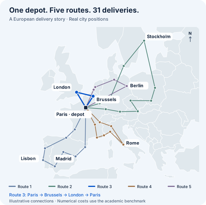
Schematic of five delivery groups on a geographic map of Europe, with Paris as the depot. Brussels lies northeast of Paris and London northwest of Brussels. Connecting lines illustrate the story, not roads or benchmark distances.

Figure 1. Geographic context for the delivery story. City positions follow real geography; straight connecting lines show illustrative visit sequences. The optimization costs below come from the benchmark, not this map. Map data: Natural Earth.

Route	Delivery stops	Crates loaded	Distance
1	8	98	230
2	10	98	267
3	2	44	59
4	7	98	155
5	4	72	73
Total	31	410	784

For a concrete view of the assignments, route 5 follows Paris → Rotterdam → Amsterdam → Hamburg → Berlin → Paris. Route 3 visits Brussels before London: Brussels is closer to Paris, and London lies west of Brussels. A real itinerary would also need road connections, Channel crossings, and driving-time constraints.

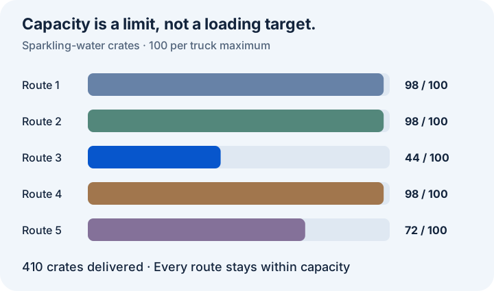
Five truck-loading bars show 98, 98, 44, 98, and 72 crates against a capacity of 100 each. Total delivered is 410 crates; route 3 retains 56 crates of unused capacity.

Figure 2. Every truck remains within capacity. Uneven loading is permitted because the objective is total distance, not equal utilization.

The 44-crate truck is a useful reminder: a less-loaded vehicle is not automatically evidence of a poor routing plan. Filling it by moving a customer from another route changes both routes’ distances. Capacity is a ceiling; equal loads are a different objective.

The follow-up, Why a Less-Loaded Truck Can Make Sense, examines that 44% loading figure, the fleet's fixed 82% departure utilization, and how to evaluate a proposed reassignment.

Worked example: the Brussels–London route

Consider route 3, which is short enough to verify by hand:

Paris depot → Brussels → London → Paris depot.

The coordinates in this calculation are the original benchmark coordinates, not the geographic positions in Figure 1.

Illustrative location	Benchmark x	Benchmark y	Crates
Paris depot	82	76	0
Brussels	61	62	24
London	57	69	20

The truck leaves with 24 + 20 = 44 crates, below its capacity of 100. It unloads 24 at Brussels, continues with 20, and returns empty after the London delivery.

The first leg has length √((82 − 61)² + (76 − 62)²) = √637, approximately 25.24, which rounds to 25. Apply the same rule to the remaining legs:

Leg	Rounded distance
Depot → Brussels	25
Brussels → London	8
London → Depot	26
Route total	59

This verifies the load and objective contribution of one route. Validating the complete plan also requires checking that all 31 destinations appear exactly once, no route exceeds 100 crates, and no more than five trucks are used.

A compact mathematical formulation

The same decisions can be expressed as a classical mixed-integer formulation. This model uses a load-based version of Miller–Tucker–Zemlin (MTZ) subtour-elimination constraints.

Let N be the customer set and V include the customers and one depot, denoted 0 in this formulation. Each customer has a positive demand qᵢ, each truck has capacity Q, at most K trucks are available, and cᵢⱼ is the cost of traveling from location i to location j. Self-arcs are excluded. In our example, there are 31 customers, Q = 100 and K = 5.

The binary variable xᵢⱼ equals 1 when a route travels directly from i to j. The continuous variable uᵢ represents cumulative demand served along a route up to customer i, including that customer's delivery; it is not the load remaining on the truck.

Minimize total travel cost:

\min \quad \sum_{i\in V}\sum_{\substack{j\in V\\j\ne i}} c_{ij}x_{ij}

Visit each customer exactly once, with one incoming and one outgoing arc. For every customer i:

\sum_{\substack{j\in V\\j\ne i}}x_{ji}=1, \qquad \sum_{\substack{j\in V\\j\ne i}}x_{ij}=1

Start and finish at the depot, using no more than K trucks:

\sum_{j\in N}x_{0j}=\sum_{i\in N}x_{i0}\le K

Respect capacity and exclude customer-only cycles. For distinct customers i and j:

u_j \ge u_i + q_j - Q(1-x_{ij})

The load bounds and variable domains are:

\begin{aligned} q_i\le u_i\le Q &\qquad (i\in N),\\ x_{ij}\in\{0,1\} &\qquad (i,j\in V,\ i\ne j). \end{aligned}

When an arc from i to j is selected, cumulative demand must increase by at least qⱼ. Its upper bound of Q limits each route's total demand. A cycle containing only customers would require cumulative demand to increase all the way around and return to its starting value—impossible with positive demands. Every route must therefore connect to the depot. The inequality is inactive when that arc is not selected.

These constraints provide a compact mathematical statement of the problem. The cited MTZ paper introduced the underlying ordering idea; the capacity interpretation here applies it to vehicle routing.

Results and verification

With a 60-second optimization budget, OptAlgo returned a feasible plan with total distance 784, matching the published best-known solution (BKS). Its deviation from BKS is therefore 0%. The academic instance and reference value are documented at the end.

The route sequences were independently checked against the original input for customer coverage, depot endpoints, fleet size, capacity, and rounded travel costs.

Result	Recorded value
Optimization budget	60 seconds
OptAlgo route distance	784
Published BKS	784
Deviation from BKS	0%
Best lower bound	Approximately 778.857
Remaining proof gap	Approximately 0.656%
Trucks used	5
Run date	September 18, 2026

A feasible objective is the cost of a valid plan: here, 784. A valid lower bound establishes a value below which the best possible objective cannot lie. Together, these values bracket the optimum for the model.

Two percentages answer different questions. Deviation from BKS compares the plan with the published reference. The proof gap compares the plan with the lower bound obtained during this run:

BKS deviation = (OptAlgo objective − BKS) / BKS × 100
              = (784 − 784) / 784 × 100 = 0%

proof gap = (feasible objective − lower bound) / feasible objective × 100
          ≈ (784 − 778.857) / 784 × 100 ≈ 0.656%

The plan matches the BKS, while the run's own lower bound leaves a small proof gap after the 60-second budget. These statements are consistent: finding a reference-quality solution and proving it optimal are separate achievements. Neither percentage measures operational savings.

For professionals, the plan illustrates the assignment and capacity decisions. For students, its two-stop route provides a checkable calculation. For researchers, reporting the optimization budget, BKS deviation, and proof gap makes the result interpretable.

Modeling choices and limitations

Minimizing total distance does not automatically balance driver workloads, minimize the longest route, or account for tolls and wages. Those goals require an explicit modeling decision. The wide range of route distances here—59 to 267—makes that distinction visible.

Likewise, a real delivery plan may need time windows, loading restrictions, driver breaks, mixed vehicle types, or travel times that change throughout the day. Straight-line benchmark distances cannot establish the quality of real city-to-city routes. One-way roads can also make travel costs asymmetric.

This example illustrates a verified result on one instance. It does not establish solve-time guarantees or expected savings for a business. Any additional constraints and supported workflow should be confirmed when defining an OptAlgo application.

Academic instance and references

Behind the delivery story is A-n32-k5, from the Set A CVRP instances attributed to Augerat et al. (1995). It contains 32 locations including the depot, vehicle capacity 100, and a five-vehicle convention. Its coordinates, demands, rounded-distance rule, and route data were preserved in the calculations. The product, city labels, and geographic illustration are editorial additions; they did not enter the optimization.

The worked route corresponds to original depot node 1 and customer nodes 25 and 28, labeled Paris, Brussels, and London. Readers can reproduce its arithmetic directly from the public instance.

CVRPLIB lists a BKS of 784, marked as optimal. The selected OptAlgo plan matches that published value after the 60-second optimization budget. The reference establishes the known optimum for this instance; the run's own lower bound retains the proof gap reported above.

Augerat et al. (1995), Set A. CVRPLIB instance collection and reference values, maintained by the research community at PUC-Rio. The original A-n32-k5 data provides the coordinates and demands. Accessed September 18, 2026.
Reinelt, G., TSPLIB 95. Documentation of distance conventions, section 2.1, and the TSPLIB FAQ on rounding and optimal solutions.
Natural Earth. Public-domain geographic data for the country outlines and city positions used in Figure 1. Geographic data is used for illustration only.
Miller, C. E., Tucker, A. W., and Zemlin, R. A. (1960). Integer Programming Formulation of Traveling Salesman Problems, Journal of the ACM, 7(4), 326–329. Foundational reference for MTZ ordering constraints.