
Explanation Routing
Why a Less-Loaded Truck Can Make Sense
A follow-up to our CVRP worked example: why one truck leaves at 44% capacity, and how to assess its role in the complete delivery plan.
In our guide to the Capacitated Vehicle Routing Problem (CVRP), five trucks deliver 410 crates of sparkling water to 31 destinations. Each truck can carry 100 crates, yet one leaves with only 44. This follow-up examines that result and asks whether moving deliveries onto the lightly loaded truck would improve the complete plan.
The truck that looks underused
The 44-crate truck uses 44% of its departure capacity, while three other trucks are almost full.
It is tempting to move more deliveries onto the lightly loaded truck. But a better-looking loading chart does not tell us whether the complete route plan improves. We need to check what changes for both the receiving truck and the truck giving up a delivery.

Figure 1. Spare capacity is visible; its effect on the full routing plan requires a calculation. This is a conceptual illustration, not a map or a scale drawing of the benchmark load.
In that model, every customer receives its entire order from one truck. Each truck makes one trip from the depot and back.
Here is the plan reported in that guide:
| Truck | Crates loaded | Departure capacity used | Route distance |
|---|---|---|---|
| 1 | 98 | 98% | 230 |
| 2 | 98 | 98% | 267 |
| 3 | 44 | 44% | 59 |
| 4 | 98 | 98% | 155 |
| 5 | 72 | 72% | 73 |
| Total | 410 | 82% across the fleet | 784 |
Distances are abstract benchmark units, not kilometres or measured road distances. The original guide explains the distance convention and assumptions.
Truck 3 stands out because it leaves with 56 crates of spare capacity. That number describes its departure load. It does not establish that another assignment would travel less.
The 90 crates of capacity that cannot disappear
Four single-trip trucks can carry at most 400 crates. With 410 crates to deliver and at most five trucks available, every feasible plan must use all five. The reported routes show that five are sufficient for this instance; the aggregate capacity calculation alone would not prove that the individual customer orders can be packed into five routes.
Once all five trucks are required, the fleet arithmetic is fixed:
| Quantity | Calculation | Result |
|---|---|---|
| Departure capacity | 5 × 100 | 500 crates |
| Demand to deliver | Sum of customer orders | 410 crates |
| Unused departure capacity | 500 − 410 | 90 crates |
| Fleet departure-load utilization | 410 ÷ 500 | 82% |
Reassigning deliveries changes which truck carries the unused capacity. It cannot change the fleet total while demand, vehicle capacities, and the number of trips remain the same.
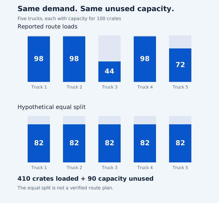
Figure 2. Redistributing a fixed load leaves the fleet total unchanged. The equal split is an arithmetic illustration; it is not a demonstrated feasible assignment of whole customer orders, and no route distance is claimed for it.
For readers who prefer the algebra, let D be total demand, Q each truck's capacity, m the number of trucks used, and Lᵣ the load on truck r. In this delivery-only, single-trip setting:
Here, m = 5, Q = 100, and D = 410, so unused capacity is always 90 crates. Even an equal allocation of 82 crates per truck, if the indivisible orders permitted it, would leave that total unchanged.
This is departure-load utilization. It does not measure how full the vehicles remain over the distance traveled, how busy the drivers are, or how much of the working day the fleet uses.
What actually changes when a delivery moves?
The guide minimizes total route distance. Capacity is a constraint; equal loading is not part of that objective.
To assess a proposed move, evaluate both affected routes:
Each change is the route's new distance minus its old distance. Keep every other route unchanged for this comparison, or include its change too.
| Total change | Meaning for the distance objective |
|---|---|
| Negative | The complete plan travels less. |
| Zero | Distance is unchanged, even if loads become more equal. |
| Positive | The complete plan travels farther. |
The receiving truck must have enough capacity, every order must still be served exactly once, and both routes must start and finish at the depot. Any additional operational constraints must also remain satisfied. Capacity availability is necessary for the move, but it does not tell us its distance effect.
The two-stop route in the original guide makes this concrete: the 44-crate truck serves two orders and contributes 59 distance units. Adding another customer requires evaluating the new visit sequence and the route that loses that customer. A loading percentage alone supplies neither calculation.
What the benchmark result establishes
The reported total of 784 matches the underlying benchmark's published optimum. Uneven departure loads therefore occur in a distance-optimal plan for this particular instance. This does not show that every unequal plan is good, that the plan is unique, or that equal loads would necessarily require more distance.
There is a separate question about the optimization run. With a 60-second optimization budget, OptAlgo matched the reference value while retaining a proof gap of approximately 0.656%. The published reference establishes the known optimum; the run did not independently close its own proof gap. The results section of the guide reports both measures.
This article interprets that existing result. It does not report a separate load-balancing experiment or claim a measured distance penalty for more equal loads.
When balance belongs in the model
Load balance can be a legitimate requirement. It needs a definition that matches the operational decision.
| Operational concern | What to represent and evaluate |
|---|---|
| One driver's day is too long | Travel time, service time, breaks, and a route-duration limit or objective |
| Physical work is uneven | Handling effort, delivery quantities, stop characteristics, and an explicit workload measure |
| Too many vehicles are being used | Vehicle-use costs or a fleet-size objective, alongside feasibility constraints |
| Trucks leave with spare capacity | Departure loading, with the fixed demand and available capacity made explicit |
These are possible modeling choices, not claims that the benchmark already includes them. Changing the objective or adding a constraint calls for a new comparison. Allowing multiple trips, using vehicles of different sizes, or changing which demand is served would also change the fleet-capacity calculation.
A lightly loaded truck is a useful reason to inspect a plan. The next step is to compare a feasible alternative against the objective that matters to the operation.
Judge the whole plan: the demand it serves, the constraints it respects, and the cost it achieves.
Academic instance and references
The example uses A-n32-k5, from the Set A instances attributed to Augerat et al. (1995). Its 31 customer demands sum to 410, and each vehicle has capacity 100. CVRPLIB lists 784 as optimal. Recalculating the public reference solution reproduces the five load-and-distance pairs in the table, with different route numbering.
The sparkling-water crates and European city labels come from the original guide's delivery story. They do not change the benchmark's coordinates, demands, or rounded Euclidean distance convention. No road-routing result is claimed.
- OptAlgo (2026). Capacitated Vehicle Routing Problem: Inputs, Constraints, and a Worked Example. Model assumptions, route calculations, and the reported 60-second result.
- Augerat et al. (1995), Set A. Original A-n32-k5 instance, distributed by CVRPLIB. Coordinates, demands, and vehicle capacity. Accessed September 19, 2026.
- CVRPLIB. A-n32-k5 reference solution and instance table with optimality status. Accessed September 19, 2026.